The Response of Interest List the Factors of Interest and Whether They Are Categorical or Continuous

Problem Statement

Let's continue the row and column percentage example from the Crosstabs tutorial, which described the relationship between the variables RankUpperUnder (upperclassman/underclassman) and LivesOnCampus (lives on campus/lives off-campus). Recall that the column percentages of the crosstab appeared to indicate that upperclassmen were less likely than underclassmen to live on campus:

• The proportion of underclassmen who live off campus is 34.8%, or 79/227.
• The proportion of underclassmen who live on campus is 65.2%, or 148/227.
• The proportion of upperclassmen who live off campus is 94.4%, or 152/161.
• The proportion of upperclassmen who live on campus is 5.6%, or 9/161.

Suppose that we want to test the association between class rank and living on campus using a Chi-Square Test of Independence (using α = 0.05).

Before the Test

The clustered bar chart from the Crosstabs procedure can act as a complement to the column percentages above. Let's look at the chart produced by the Crosstabs procedure for this example:

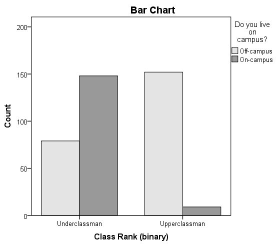
The height of each bar represents the total number of observations in that particular combination of categories. The "clusters" are formed by the row variable (in this case, class rank). This type of chart emphasizes the differences within the underclassmen and upperclassmen groups. Here, the differences in number of students living on campus versus living off-campus is much starker within the class rank groups.

Running the Test

1. Open the Crosstabs dialog (Analyze > Descriptive Statistics > Crosstabs).
2. Select RankUpperUnder as the row variable, and LiveOnCampus as the column variable.
3. Click Statistics. Check Chi-square, then click Continue.
4. (Optional) Click Cells. Under Counts, check the boxes for Observed and Expected, and under Residuals, click Unstandardized. Then click Continue.
5. (Optional) Check the box for Display clustered bar charts.
6. Click OK.

Output

Syntax

          CROSSTABS   /TABLES=RankUpperUnder BY LiveOnCampus   /FORMAT=AVALUE TABLES   /STATISTICS=CHISQ    /CELLS=COUNT EXPECTED RESID    /COUNT ROUND CELL   /BARCHART.        

Tables

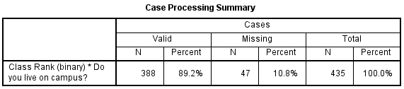
The first table is the Case Processing summary, which tells us the number of valid cases used for analysis. Only cases with nonmissing values for both class rank and living on campus can be used in the test.

The next table is the crosstabulation. If you elected to check off the boxes for Observed Count, Expected Count, and Unstandardized Residuals, you should see the following table:

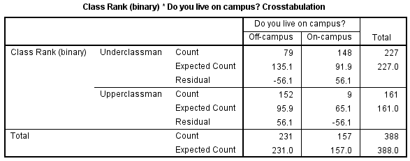
With the Expected Count values shown, we can confirm that all cells have an expected value greater than 5.

Computation of the expected cell counts and residuals (observed minus expected) for the crosstabulation of class rank by living on campus.

	Off-Campus	On-Campus	Total
Underclassman	Row 1, column 1 $$ o_{\mathrm{11}} = 79 $$ $$ e_{\mathrm{11}} = \frac{227*231}{388} = 135.147 $$ $$ r_{\mathrm{11}} = 79 - 135.147 = -56.147 $$	Row 1, column 2 $$ o_{\mathrm{12}} = 148 $$ $$ e_{\mathrm{12}} = \frac{227*157}{388} = 91.853 $$ $$ r_{\mathrm{12}} = 148 - 91.853 = 56.147 $$	row 1 total = 227
Upperclassmen	Row 2, column 1 $$ o_{\mathrm{21}} = 152 $$ $$ e_{\mathrm{21}} = \frac{161*231}{388} = 95.853 $$ $$ r_{\mathrm{21}} = 152 - 95.853 = 56.147 $$	Row 2, column 2 $$ o_{\mathrm{22}} = 9 $$ $$ e_{\mathrm{22}} = \frac{161*157}{388} = 65.147 $$ $$ r_{\mathrm{22}} = 9 - 65.147 = -56.147 $$	row 2 total = 161
Total	col 1 total = 231	col 2 total = 157	grand total = 388

These numbers can be plugged into the chi-square test statistic formula:

$$ \chi^{2} = \sum_{i=1}^{R}{\sum_{j=1}^{C}{\frac{(o_{ij} - e_{ij})^{2}}{e_{ij}}}} = \frac{(-56.147)^{2}}{135.147} + \frac{(56.147)^{2}}{91.853} + \frac{(56.147)^{2}}{95.853} + \frac{(-56.147)^{2}}{65.147} = 138.926 $$

We can confirm this computation with the results in the Chi-Square Tests table:

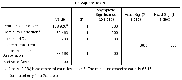
The row of interest here is Pearson Chi-Square and its footnote.

• The value of the test statistic is 138.926.
• The footnote for this statistic pertains to the expected cell count assumption (i.e., expected cell counts are all greater than 5): no cells had an expected count less than 5, so this assumption was met.
• Because the crosstabulation is a 2x2 table, the degrees of freedom (df) for the test statistic is $$ df = (R - 1)*(C - 1) = (2 - 1)*(2 - 1) = 1 $$.
• The corresponding p-value of the test statistic is so small that it is cut off from display. Instead of writing "p = 0.000", we instead write the mathematically correct statement p < 0.001.

Decision and Conclusions

Since the p-value is less than our chosen significance level α = 0.05, we can reject the null hypothesis, and conclude that there is an association between class rank and whether or not students live on-campus.

Based on the results, we can state the following:

• There was a significant association between class rank and living on campus (Χ ²(1) = 138.9, p < .001).

mcdonnellhiscambeste.blogspot.com

Source: https://libguides.library.kent.edu/spss/chisquare

Share this post